| PX_ID | min_list_date | previous_TX | dialysis | waitlist_end_date | diabetes | age_months | CAN_DIAL_DT | dialysis_time_at_list | wait_time |
|---|---|---|---|---|---|---|---|---|---|
| 1 | 2015-09-03 | 0 | 0 | 2016-02-09 | 0 | 713 | 2015-11-15 | 0 | 159 days |
| 2 | 2012-02-03 | 0 | 1 | 2012-04-16 | 0 | 439 | 2011-09-20 | 136 | 73 days |
| 3 | 2014-04-30 | 1 | 0 | 2014-12-20 | 0 | 339 | NA | 0 | 234 days |
| 4 | 2012-07-01 | 0 | 1 | 2015-01-01 | 0 | 654 | 2011-07-01 | 366 | 914 days |
| 5 | 2012-07-01 | 0 | 0 | 2015-01-01 | 0 | 654 | 2013-01-01 | 0 | 914 days |
| 6 | 2012-07-01 | 0 | 0 | 2015-01-01 | 0 | 654 | NA | 0 | 914 days |
Time Varying EPTS
Data Structures
Kidney Allocation
R
In the SRTR Standard Analysis Files, the CAND_KIPA file includes information on candidates listed for kidney and/or pancreas transplants. From this file, it is possible to calculate a candidate EPTS score at listing, but it does not directly account for the change in dialysis time and age during a patient’s time on the waitlist that can lead to higher EPTS scores over time. To perform analyses on EPTS scores that change over time, it is possible to request an enhanced SAF from the SRTR that includes time-varying EPTS. Alternatively, you can consctruct a discrete time dataset that can be used to calculate EPTS at different periods during a candidate’s time on the waitlist. In this post we will address how we constructed such a dataset for our manuscript Association of Race and Ethnicity with Priority for Deceased Donor Kidney Transplant.
Let’s take a look at our data:
Note
These data are fabricated and do not represent real patients listed for kidney transplant
PX_ID is a unique patient identifier
min_list_date is the earliest date a patient is listed for a transplant. This takes into account patients who are listed at multiple centers concurrently. We will explain how to address such patients in another post.
previous_TX is an indicator for whether the patient has received a previous transplant
dialysis is an indicator for whether the patient was on dialysis when they were listed
waitlist_end_date is the date that the patient received a transplant or was otherwise removed from the waiting list
diabetes is an indicator for whether the candidate has diabetes
age_months is the candidate’s age in months at listing
CAN_DIAL_DT is the date the candidate started dialysis (if at all)
dialysis_time_at_list is how long the patient was on dialysis before being placed on the waitlist
wait_time is the time between the candidate’s listing and their waitlist end date
With these variables we would be able to calculate a patient’s EPTS score at listing, but neither the age nor dialysis time variable captures changes over time. To address this, we can create a discrete time data set with 1 month intervals such that the age and dialysis time increase every month that the candidate is on the waitlist.
First, we will flag patient’s who were pre-emptively listed and then started dialysis during their time on the waitlist:
df_epts_varying$dialysis_during_waitlist <- ifelse(df_epts_varying$CAN_DIAL_DT > df_epts_varying$min_list_date, 1, 0)
df_epts_varying$dialysis_during_waitlist[is.na(df_epts_varying$dialysis_during_waitlist)] <- 0
We will then calculate the total months that each patient was on the waitlist:
df_epts_varying = df_epts_varying %>% mutate(time_period = as.integer(floor((wait_time)*12/365)))To properly encode the dialysis time for patients who begin dialysis after listing, we use a time_until_dialysis variable, which we will later compare to the patient’s time on the waitlist to trigger the dialysis_time variable to start increasing
df_epts_varying = df_epts_varying %>% mutate(time_until_dialysis = ifelse(dialysis_during_waitlist == 1, as.integer(floor((CAN_DIAL_DT - min_list_date)*12/365)), 0))Using the time period variable, we construct a dataset which has an observation for each month the patient is on the waitlist.
expanded_data <- df_epts_varying %>%
  tidyr::uncount(weights = time_period + 1) %>%
  group_by(PX_ID) %>%
  mutate(time = ifelse(row_number() <= time_period + 1, row_number() - 1, NA),
    time = ifelse(is.na(time), max(time, na.rm = TRUE), time),
    age = age_months/12
  ) %>%
  mutate(age = age + row_number()/12)

expanded_data = expanded_data %>%
  mutate(dialysis_after_waitlist = case_when(
    dialysis_during_waitlist == 1 & (time - time_until_dialysis) < 0 ~ 0,
    dialysis_during_waitlist == 1 & (time - time_until_dialysis) >= 0 ~ (time - time_until_dialysis),
    dialysis_during_waitlist == 0 & dialysis == 1 ~ (time - time_until_dialysis),
    TRUE ~ 0))

expanded_data = expanded_data %>% mutate(dialysis_time = dialysis_time_at_list + dialysis_after_waitlist/12)
As we can see below, this process allows us to determine dialysis time and age at each month of a patient’s time on the waitlist in order to accurately calculate EPTS at each time step
| PX_ID | time | dialysis_time_at_list | dialysis_after_waitlist | dialysis_time | age |
|---|---|---|---|---|---|
| 1 | 0 | 0 | 0 | 0.0000000 | 59.50000 |
| 1 | 1 | 0 | 0 | 0.0000000 | 59.58333 |
| 1 | 2 | 0 | 0 | 0.0000000 | 59.66667 |
| 1 | 3 | 0 | 1 | 0.0833333 | 59.75000 |
| 1 | 4 | 0 | 2 | 0.1666667 | 59.83333 |
| 1 | 5 | 0 | 3 | 0.2500000 | 59.91667 |
| 2 | 0 | 136 | 0 | 136.0000000 | 36.66667 |
| 2 | 1 | 136 | 1 | 136.0833333 | 36.75000 |
| 2 | 2 | 136 | 2 | 136.1666667 | 36.83333 |
| 3 | 0 | 0 | 0 | 0.0000000 | 28.33333 |
| 3 | 1 | 0 | 0 | 0.0000000 | 28.41667 |
| 3 | 2 | 0 | 0 | 0.0000000 | 28.50000 |
| 3 | 3 | 0 | 0 | 0.0000000 | 28.58333 |
| 3 | 4 | 0 | 0 | 0.0000000 | 28.66667 |
| 3 | 5 | 0 | 0 | 0.0000000 | 28.75000 |
| 3 | 6 | 0 | 0 | 0.0000000 | 28.83333 |
| 3 | 7 | 0 | 0 | 0.0000000 | 28.91667 |
| 4 | 0 | 366 | 0 | 366.0000000 | 54.58333 |
| 4 | 1 | 366 | 1 | 366.0833333 | 54.66667 |
| 4 | 2 | 366 | 2 | 366.1666667 | 54.75000 |
| 4 | 3 | 366 | 3 | 366.2500000 | 54.83333 |
| 4 | 4 | 366 | 4 | 366.3333333 | 54.91667 |
| 4 | 5 | 366 | 5 | 366.4166667 | 55.00000 |
| 4 | 6 | 366 | 6 | 366.5000000 | 55.08333 |
| 4 | 7 | 366 | 7 | 366.5833333 | 55.16667 |
| 4 | 8 | 366 | 8 | 366.6666667 | 55.25000 |
| 4 | 9 | 366 | 9 | 366.7500000 | 55.33333 |
| 4 | 10 | 366 | 10 | 366.8333333 | 55.41667 |
| 4 | 11 | 366 | 11 | 366.9166667 | 55.50000 |
| 4 | 12 | 366 | 12 | 367.0000000 | 55.58333 |
| 4 | 13 | 366 | 13 | 367.0833333 | 55.66667 |
| 4 | 14 | 366 | 14 | 367.1666667 | 55.75000 |
| 4 | 15 | 366 | 15 | 367.2500000 | 55.83333 |
| 4 | 16 | 366 | 16 | 367.3333333 | 55.91667 |
| 4 | 17 | 366 | 17 | 367.4166667 | 56.00000 |
| 4 | 18 | 366 | 18 | 367.5000000 | 56.08333 |
| 4 | 19 | 366 | 19 | 367.5833333 | 56.16667 |
| 4 | 20 | 366 | 20 | 367.6666667 | 56.25000 |
| 4 | 21 | 366 | 21 | 367.7500000 | 56.33333 |
| 4 | 22 | 366 | 22 | 367.8333333 | 56.41667 |
| 4 | 23 | 366 | 23 | 367.9166667 | 56.50000 |
| 4 | 24 | 366 | 24 | 368.0000000 | 56.58333 |
| 4 | 25 | 366 | 25 | 368.0833333 | 56.66667 |
| 4 | 26 | 366 | 26 | 368.1666667 | 56.75000 |
| 4 | 27 | 366 | 27 | 368.2500000 | 56.83333 |
| 4 | 28 | 366 | 28 | 368.3333333 | 56.91667 |
| 4 | 29 | 366 | 29 | 368.4166667 | 57.00000 |
| 4 | 30 | 366 | 30 | 368.5000000 | 57.08333 |
| 5 | 0 | 0 | 0 | 0.0000000 | 54.58333 |
| 5 | 1 | 0 | 0 | 0.0000000 | 54.66667 |
| 5 | 2 | 0 | 0 | 0.0000000 | 54.75000 |
| 5 | 3 | 0 | 0 | 0.0000000 | 54.83333 |
| 5 | 4 | 0 | 0 | 0.0000000 | 54.91667 |
| 5 | 5 | 0 | 0 | 0.0000000 | 55.00000 |
| 5 | 6 | 0 | 0 | 0.0000000 | 55.08333 |
| 5 | 7 | 0 | 1 | 0.0833333 | 55.16667 |
| 5 | 8 | 0 | 2 | 0.1666667 | 55.25000 |
| 5 | 9 | 0 | 3 | 0.2500000 | 55.33333 |
| 5 | 10 | 0 | 4 | 0.3333333 | 55.41667 |
| 5 | 11 | 0 | 5 | 0.4166667 | 55.50000 |
| 5 | 12 | 0 | 6 | 0.5000000 | 55.58333 |
| 5 | 13 | 0 | 7 | 0.5833333 | 55.66667 |
| 5 | 14 | 0 | 8 | 0.6666667 | 55.75000 |
| 5 | 15 | 0 | 9 | 0.7500000 | 55.83333 |
| 5 | 16 | 0 | 10 | 0.8333333 | 55.91667 |
| 5 | 17 | 0 | 11 | 0.9166667 | 56.00000 |
| 5 | 18 | 0 | 12 | 1.0000000 | 56.08333 |
| 5 | 19 | 0 | 13 | 1.0833333 | 56.16667 |
| 5 | 20 | 0 | 14 | 1.1666667 | 56.25000 |
| 5 | 21 | 0 | 15 | 1.2500000 | 56.33333 |
| 5 | 22 | 0 | 16 | 1.3333333 | 56.41667 |
| 5 | 23 | 0 | 17 | 1.4166667 | 56.50000 |
| 5 | 24 | 0 | 18 | 1.5000000 | 56.58333 |
| 5 | 25 | 0 | 19 | 1.5833333 | 56.66667 |
| 5 | 26 | 0 | 20 | 1.6666667 | 56.75000 |
| 5 | 27 | 0 | 21 | 1.7500000 | 56.83333 |
| 5 | 28 | 0 | 22 | 1.8333333 | 56.91667 |
| 5 | 29 | 0 | 23 | 1.9166667 | 57.00000 |
| 5 | 30 | 0 | 24 | 2.0000000 | 57.08333 |
| 6 | 0 | 0 | 0 | 0.0000000 | 54.58333 |
| 6 | 1 | 0 | 0 | 0.0000000 | 54.66667 |
| 6 | 2 | 0 | 0 | 0.0000000 | 54.75000 |
| 6 | 3 | 0 | 0 | 0.0000000 | 54.83333 |
| 6 | 4 | 0 | 0 | 0.0000000 | 54.91667 |
| 6 | 5 | 0 | 0 | 0.0000000 | 55.00000 |
| 6 | 6 | 0 | 0 | 0.0000000 | 55.08333 |
| 6 | 7 | 0 | 0 | 0.0000000 | 55.16667 |
| 6 | 8 | 0 | 0 | 0.0000000 | 55.25000 |
| 6 | 9 | 0 | 0 | 0.0000000 | 55.33333 |
| 6 | 10 | 0 | 0 | 0.0000000 | 55.41667 |
| 6 | 11 | 0 | 0 | 0.0000000 | 55.50000 |
| 6 | 12 | 0 | 0 | 0.0000000 | 55.58333 |
| 6 | 13 | 0 | 0 | 0.0000000 | 55.66667 |
| 6 | 14 | 0 | 0 | 0.0000000 | 55.75000 |
| 6 | 15 | 0 | 0 | 0.0000000 | 55.83333 |
| 6 | 16 | 0 | 0 | 0.0000000 | 55.91667 |
| 6 | 17 | 0 | 0 | 0.0000000 | 56.00000 |
| 6 | 18 | 0 | 0 | 0.0000000 | 56.08333 |
| 6 | 19 | 0 | 0 | 0.0000000 | 56.16667 |
| 6 | 20 | 0 | 0 | 0.0000000 | 56.25000 |
| 6 | 21 | 0 | 0 | 0.0000000 | 56.33333 |
| 6 | 22 | 0 | 0 | 0.0000000 | 56.41667 |
| 6 | 23 | 0 | 0 | 0.0000000 | 56.50000 |
| 6 | 24 | 0 | 0 | 0.0000000 | 56.58333 |
| 6 | 25 | 0 | 0 | 0.0000000 | 56.66667 |
| 6 | 26 | 0 | 0 | 0.0000000 | 56.75000 |
| 6 | 27 | 0 | 0 | 0.0000000 | 56.83333 |
| 6 | 28 | 0 | 0 | 0.0000000 | 56.91667 |
| 6 | 29 | 0 | 0 | 0.0000000 | 57.00000 |
| 6 | 30 | 0 | 0 | 0.0000000 | 57.08333 |
Each patient’s raw EPTS score is calculated using the following formula:
Raw EPTS = 0.047*max(Age-25,0)- 0.015*Diabetes*max(Age-25,0) \\ + 0.398*Prior Organ Transplant - 0.237*Diabetes*Prior Organ Transplant \\ + 0.315*log(Dialysis Time + 1) - 0.099*Diabetes*log(Dialysis Time + 1) \\+ 0.130*(Dialysis Time = 0) - 0.348*Diabetes*(Dialysis Time = 0) + 1.262*Diabetes
We then use the EPTS mapping table from 2021 shown here to calculate EPTS of these patients at each month on the waitlist.
| 0.0000000 | 1.842390e-02 | 0 |
| 0.0184239 | 2.358706e-01 | 1 |
| 0.2358706 | 4.188522e-01 | 2 |
| 0.4188522 | 5.280000e-01 | 3 |
| 0.5280000 | 6.285256e-01 | 4 |
| 0.6285256 | 7.135270e-01 | 5 |
| 0.7135270 | 7.922030e-01 | 6 |
| 0.7922030 | 8.671443e-01 | 7 |
| 0.8671443 | 9.304798e-01 | 8 |
| 0.9304798 | 9.939185e-01 | 9 |
| 0.9939185 | 1.055990e+00 | 10 |
| 1.0559898 | 1.114348e+00 | 11 |
| 1.1143479 | 1.170456e+00 | 12 |
| 1.1704557 | 1.220301e+00 | 13 |
| 1.2203005 | 1.272125e+00 | 14 |
| 1.2721250 | 1.319138e+00 | 15 |
| 1.3191377 | 1.364385e+00 | 16 |
| 1.3643854 | 1.411682e+00 | 17 |
| 1.4116824 | 1.454332e+00 | 18 |
| 1.4543320 | 1.494737e+00 | 19 |
| 1.4947372 | 1.535142e+00 | 20 |
| 1.5351424 | 1.573005e+00 | 21 |
| 1.5730051 | 1.608103e+00 | 22 |
| 1.6081034 | 1.642976e+00 | 23 |
| 1.6429760 | 1.673541e+00 | 24 |
| 1.6735411 | 1.702554e+00 | 25 |
| 1.7025537 | 1.731507e+00 | 26 |
| 1.7315065 | 1.758694e+00 | 27 |
| 1.7586938 | 1.784780e+00 | 28 |
| 1.7847796 | 1.811802e+00 | 29 |
| 1.8118022 | 1.836835e+00 | 30 |
| 1.8368350 | 1.860602e+00 | 31 |
| 1.8606023 | 1.883752e+00 | 32 |
| 1.8837516 | 1.907272e+00 | 33 |
| 1.9072723 | 1.929411e+00 | 34 |
| 1.9294107 | 1.951500e+00 | 35 |
| 1.9514996 | 1.973708e+00 | 36 |
| 1.9737084 | 1.994142e+00 | 37 |
| 1.9941416 | 2.014865e+00 | 38 |
| 2.0148654 | 2.033233e+00 | 39 |
| 2.0332331 | 2.053976e+00 | 40 |
| 2.0539760 | 2.073276e+00 | 41 |
| 2.0732762 | 2.092022e+00 | 42 |
| 2.0920218 | 2.110557e+00 | 43 |
| 2.1105572 | 2.127109e+00 | 44 |
| 2.1271095 | 2.144695e+00 | 45 |
| 2.1446947 | 2.162066e+00 | 46 |
| 2.1620664 | 2.178958e+00 | 47 |
| 2.1789580 | 2.195336e+00 | 48 |
| 2.1953362 | 2.212030e+00 | 49 |
| 2.2120298 | 2.228307e+00 | 50 |
| 2.2283066 | 2.244865e+00 | 51 |
| 2.2448652 | 2.259348e+00 | 52 |
| 2.2593477 | 2.274579e+00 | 53 |
| 2.2745791 | 2.290074e+00 | 54 |
| 2.2900737 | 2.305555e+00 | 55 |
| 2.3055553 | 2.321628e+00 | 56 |
| 2.3216283 | 2.336763e+00 | 57 |
| 2.3367630 | 2.352642e+00 | 58 |
| 2.3526424 | 2.368047e+00 | 59 |
| 2.3680465 | 2.382880e+00 | 60 |
| 2.3828801 | 2.397443e+00 | 61 |
| 2.3974431 | 2.411764e+00 | 62 |
| 2.4117645 | 2.426611e+00 | 63 |
| 2.4266108 | 2.441439e+00 | 64 |
| 2.4414390 | 2.456166e+00 | 65 |
| 2.4561660 | 2.470464e+00 | 66 |
| 2.4704641 | 2.485417e+00 | 67 |
| 2.4854167 | 2.500826e+00 | 68 |
| 2.5008259 | 2.515759e+00 | 69 |
| 2.5157591 | 2.531790e+00 | 70 |
| 2.5317904 | 2.548471e+00 | 71 |
| 2.5484715 | 2.564502e+00 | 72 |
| 2.5645021 | 2.580563e+00 | 73 |
| 2.5805634 | 2.596225e+00 | 74 |
| 2.5962254 | 2.612206e+00 | 75 |
| 2.6122058 | 2.629802e+00 | 76 |
| 2.6298023 | 2.646337e+00 | 77 |
| 2.6463374 | 2.662708e+00 | 78 |
| 2.6627084 | 2.680714e+00 | 79 |
| 2.6807143 | 2.699657e+00 | 80 |
| 2.6996572 | 2.719246e+00 | 81 |
| 2.7192464 | 2.738536e+00 | 82 |
| 2.7385362 | 2.757782e+00 | 83 |
| 2.7577815 | 2.777288e+00 | 84 |
| 2.7772876 | 2.797192e+00 | 85 |
| 2.7971922 | 2.818845e+00 | 86 |
| 2.8188454 | 2.839567e+00 | 87 |
| 2.8395672 | 2.861173e+00 | 88 |
| 2.8611734 | 2.884584e+00 | 89 |
| 2.8845836 | 2.906797e+00 | 90 |
| 2.9067967 | 2.931876e+00 | 91 |
| 2.9318760 | 2.955637e+00 | 92 |
| 2.9556373 | 2.981927e+00 | 93 |
| 2.9819266 | 3.010420e+00 | 94 |
| 3.0104196 | 3.042116e+00 | 95 |
| 3.0421156 | 3.076537e+00 | 96 |
| 3.0765369 | 3.118385e+00 | 97 |
| 3.1183851 | 3.171600e+00 | 98 |
| 3.1715997 | 3.248494e+00 | 99 |
| 3.2484942 | 1.000000e+09 | 100 |
This results in our final dataset which includes each EPTS variable and the resulting EPTS score for each month a patient is on the wailist.
| PX_ID | Age | Dialysis Time | Previous TX | Diabetes | Percentile EPTS |
|---|---|---|---|---|---|
| 1 | 59.50000 | 0.0000000 | 0 | 0 | 27 |
| 1 | 59.58333 | 0.0000000 | 0 | 0 | 27 |
| 1 | 59.66667 | 0.0000000 | 0 | 0 | 28 |
| 1 | 59.75000 | 0.0833333 | 0 | 0 | 24 |
| 1 | 59.83333 | 0.1666667 | 0 | 0 | 25 |
| 1 | 59.91667 | 0.2500000 | 0 | 0 | 26 |
| 2 | 36.66667 | 136.0000000 | 0 | 0 | 43 |
| 2 | 36.75000 | 136.0833333 | 0 | 0 | 43 |
| 2 | 36.83333 | 136.1666667 | 0 | 0 | 43 |
| 3 | 28.33333 | 0.0000000 | 1 | 0 | 5 |
| 3 | 28.41667 | 0.0000000 | 1 | 0 | 5 |
| 3 | 28.50000 | 0.0000000 | 1 | 0 | 5 |
| 3 | 28.58333 | 0.0000000 | 1 | 0 | 5 |
| 3 | 28.66667 | 0.0000000 | 1 | 0 | 5 |
| 3 | 28.75000 | 0.0000000 | 1 | 0 | 5 |
| 3 | 28.83333 | 0.0000000 | 1 | 0 | 5 |
| 3 | 28.91667 | 0.0000000 | 1 | 0 | 5 |
| 4 | 54.58333 | 366.0000000 | 0 | 0 | 100 |
| 4 | 54.66667 | 366.0833333 | 0 | 0 | 100 |
| 4 | 54.75000 | 366.1666667 | 0 | 0 | 100 |
| 4 | 54.83333 | 366.2500000 | 0 | 0 | 100 |
| 4 | 54.91667 | 366.3333333 | 0 | 0 | 100 |
| 4 | 55.00000 | 366.4166667 | 0 | 0 | 100 |
| 4 | 55.08333 | 366.5000000 | 0 | 0 | 100 |
| 4 | 55.16667 | 366.5833333 | 0 | 0 | 100 |
| 4 | 55.25000 | 366.6666667 | 0 | 0 | 100 |
| 4 | 55.33333 | 366.7500000 | 0 | 0 | 100 |
| 4 | 55.41667 | 366.8333333 | 0 | 0 | 100 |
| 4 | 55.50000 | 366.9166667 | 0 | 0 | 100 |
| 4 | 55.58333 | 367.0000000 | 0 | 0 | 100 |
| 4 | 55.66667 | 367.0833333 | 0 | 0 | 100 |
| 4 | 55.75000 | 367.1666667 | 0 | 0 | 100 |
| 4 | 55.83333 | 367.2500000 | 0 | 0 | 100 |
| 4 | 55.91667 | 367.3333333 | 0 | 0 | 100 |
| 4 | 56.00000 | 367.4166667 | 0 | 0 | 100 |
| 4 | 56.08333 | 367.5000000 | 0 | 0 | 100 |
| 4 | 56.16667 | 367.5833333 | 0 | 0 | 100 |
| 4 | 56.25000 | 367.6666667 | 0 | 0 | 100 |
| 4 | 56.33333 | 367.7500000 | 0 | 0 | 100 |
| 4 | 56.41667 | 367.8333333 | 0 | 0 | 100 |
| 4 | 56.50000 | 367.9166667 | 0 | 0 | 100 |
| 4 | 56.58333 | 368.0000000 | 0 | 0 | 100 |
| 4 | 56.66667 | 368.0833333 | 0 | 0 | 100 |
| 4 | 56.75000 | 368.1666667 | 0 | 0 | 100 |
| 4 | 56.83333 | 368.2500000 | 0 | 0 | 100 |
| 4 | 56.91667 | 368.3333333 | 0 | 0 | 100 |
| 4 | 57.00000 | 368.4166667 | 0 | 0 | 100 |
| 4 | 57.08333 | 368.5000000 | 0 | 0 | 100 |
| 5 | 54.58333 | 0.0000000 | 0 | 0 | 20 |
| 5 | 54.66667 | 0.0000000 | 0 | 0 | 20 |
| 5 | 54.75000 | 0.0000000 | 0 | 0 | 20 |
| 5 | 54.83333 | 0.0000000 | 0 | 0 | 20 |
| 5 | 54.91667 | 0.0000000 | 0 | 0 | 21 |
| 5 | 55.00000 | 0.0000000 | 0 | 0 | 21 |
| 5 | 55.08333 | 0.0000000 | 0 | 0 | 21 |
| 5 | 55.16667 | 0.0833333 | 0 | 0 | 18 |
| 5 | 55.25000 | 0.1666667 | 0 | 0 | 19 |
| 5 | 55.33333 | 0.2500000 | 0 | 0 | 20 |
| 5 | 55.41667 | 0.3333333 | 0 | 0 | 20 |
| 5 | 55.50000 | 0.4166667 | 0 | 0 | 21 |
| 5 | 55.58333 | 0.5000000 | 0 | 0 | 21 |
| 5 | 55.66667 | 0.5833333 | 0 | 0 | 22 |
| 5 | 55.75000 | 0.6666667 | 0 | 0 | 22 |
| 5 | 55.83333 | 0.7500000 | 0 | 0 | 23 |
| 5 | 55.91667 | 0.8333333 | 0 | 0 | 24 |
| 5 | 56.00000 | 0.9166667 | 0 | 0 | 24 |
| 5 | 56.08333 | 1.0000000 | 0 | 0 | 25 |
| 5 | 56.16667 | 1.0833333 | 0 | 0 | 25 |
| 5 | 56.25000 | 1.1666667 | 0 | 0 | 26 |
| 5 | 56.33333 | 1.2500000 | 0 | 0 | 26 |
| 5 | 56.41667 | 1.3333333 | 0 | 0 | 27 |
| 5 | 56.50000 | 1.4166667 | 0 | 0 | 27 |
| 5 | 56.58333 | 1.5000000 | 0 | 0 | 28 |
| 5 | 56.66667 | 1.5833333 | 0 | 0 | 29 |
| 5 | 56.75000 | 1.6666667 | 0 | 0 | 29 |
| 5 | 56.83333 | 1.7500000 | 0 | 0 | 30 |
| 5 | 56.91667 | 1.8333333 | 0 | 0 | 30 |
| 5 | 57.00000 | 1.9166667 | 0 | 0 | 31 |
| 5 | 57.08333 | 2.0000000 | 0 | 0 | 31 |
| 6 | 54.58333 | 0.0000000 | 0 | 0 | 20 |
| 6 | 54.66667 | 0.0000000 | 0 | 0 | 20 |
| 6 | 54.75000 | 0.0000000 | 0 | 0 | 20 |
| 6 | 54.83333 | 0.0000000 | 0 | 0 | 20 |
| 6 | 54.91667 | 0.0000000 | 0 | 0 | 21 |
| 6 | 55.00000 | 0.0000000 | 0 | 0 | 21 |
| 6 | 55.08333 | 0.0000000 | 0 | 0 | 21 |
| 6 | 55.16667 | 0.0000000 | 0 | 0 | 21 |
| 6 | 55.25000 | 0.0000000 | 0 | 0 | 21 |
| 6 | 55.33333 | 0.0000000 | 0 | 0 | 21 |
| 6 | 55.41667 | 0.0000000 | 0 | 0 | 21 |
| 6 | 55.50000 | 0.0000000 | 0 | 0 | 21 |
| 6 | 55.58333 | 0.0000000 | 0 | 0 | 21 |
| 6 | 55.66667 | 0.0000000 | 0 | 0 | 21 |
| 6 | 55.75000 | 0.0000000 | 0 | 0 | 22 |
| 6 | 55.83333 | 0.0000000 | 0 | 0 | 22 |
| 6 | 55.91667 | 0.0000000 | 0 | 0 | 22 |
| 6 | 56.00000 | 0.0000000 | 0 | 0 | 22 |
| 6 | 56.08333 | 0.0000000 | 0 | 0 | 22 |
| 6 | 56.16667 | 0.0000000 | 0 | 0 | 22 |
| 6 | 56.25000 | 0.0000000 | 0 | 0 | 22 |
| 6 | 56.33333 | 0.0000000 | 0 | 0 | 22 |
| 6 | 56.41667 | 0.0000000 | 0 | 0 | 22 |
| 6 | 56.50000 | 0.0000000 | 0 | 0 | 23 |
| 6 | 56.58333 | 0.0000000 | 0 | 0 | 23 |
| 6 | 56.66667 | 0.0000000 | 0 | 0 | 23 |
| 6 | 56.75000 | 0.0000000 | 0 | 0 | 23 |
| 6 | 56.83333 | 0.0000000 | 0 | 0 | 23 |
| 6 | 56.91667 | 0.0000000 | 0 | 0 | 23 |
| 6 | 57.00000 | 0.0000000 | 0 | 0 | 23 |
| 6 | 57.08333 | 0.0000000 | 0 | 0 | 23 |
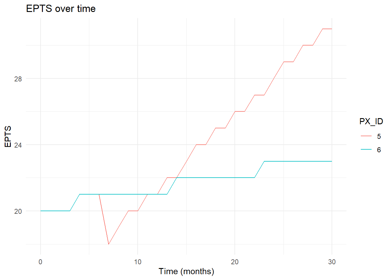
Patients 5 and 6 are an example of two patients who have the same EPTS characteristics but one patient is put on dialysis and the other is not. As we can see here, when patient 5 is put on dialysis it initially lowers their EPTS, but their EPTS soon increases to its previous level and then continues to increase at a much faster pace than patient 6 who is not on dialysis.
save(df_months, file = "time_varying_data.Rdata")